Solving Blackjack
Introduction
In this tutorial, we’ll explore and solve the Blackjack-v1 environment
(this means we’ll have an agent learn an optimal policy).
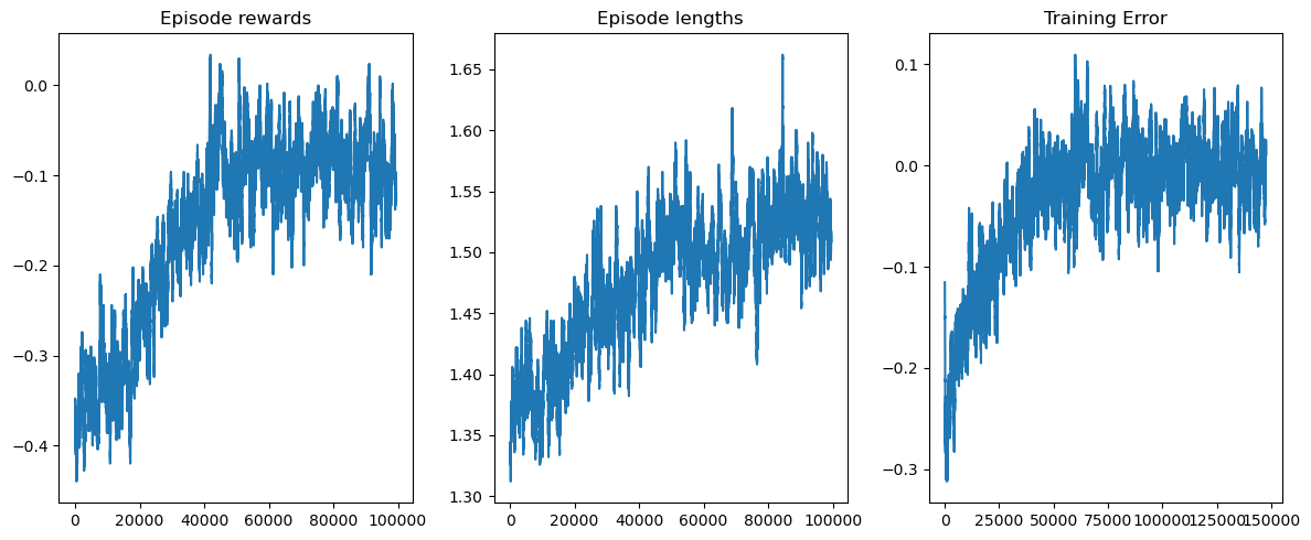
This tutorial is part of the Gymnasium documentation. A more detailed version with training plots can be found on the Gymnasium website.
The documentation for the blackjack environment is available here.
Blackjack is one of the most popular casino card games that is also infamous for being beatable under certain conditions. This version of the game uses an infinite deck (we draw the cards with replacement), so counting cards won’t be a viable strategy in our simulated game.
Objective: To win, your card sum should be greater than than the dealers without exceeding 21.
Approach: To solve this environment by yourself, you can pick your favorite discrete RL algorithm. The presented solution uses Q-learning (a model-free RL algorithm).
# Imports and Environment Setup

# Author: Till Zemann
# License: MIT License

import gymnasium as gym
import numpy as np
import matplotlib
import seaborn as sns
from matplotlib import pyplot as plt
from matplotlib.patches import Patch
from collections import defaultdict

matplotlib.use('TkAgg')
plt.rcParams['text.usetex'] = True

# Let's start by creating the blackjack environment.
# Note: We are going to follow the rules from Sutton & Barto.
# Other versions of the game can be found below for you to experiment.

env = gym.make('Blackjack-v1', sab=True)
Other possible environment configurations:
env = gym.make('Blackjack-v1', natural=True, sab=False)
env = gym.make('Blackjack-v1', natural=False, sab=False)
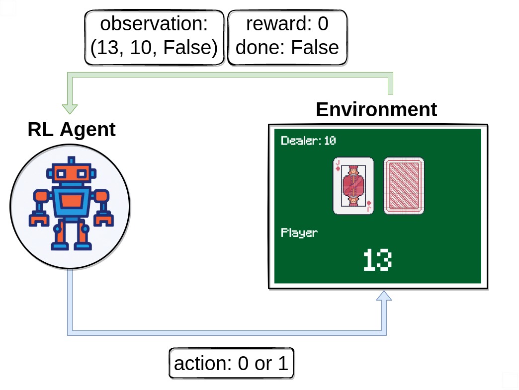
Basics: Interacting with the environment
Observing the environment
First of all, we call env.reset() to start an episode. This function
resets the environment to a starting position and returns an initial
observation. We usually also set done = False. This variable
will be useful later to check if a game is terminated. In this tutorial
we will use the terms observation and state synonymously but in more
complex problems a state might differ from the observation it is based
on.
# reset the environment to get the first observation
done = False
observation, info = env.reset()

print(observation)
Note that our observation is a 3-tuple consisting of 3 discrete values:
- The players current sum
- Value of the dealers face-up card
- Boolean whether the player holds a usable ace (An ace is usable if it counts as 11 without busting)
Executing an action
After receiving our first observation, we are only going to use the
env.step(action) function to interact with the environment. This
function takes an action as input and executes it in the environment.
Because that action changes the state of the environment, it returns
four useful variables to us. These are:
next_state: This is the observation that the agent will receive after taking the action.reward: This is the reward that the agent will receive after taking the action.terminated: This is a boolean variable that indicates whether or not the episode is over.truncated: This is a boolean variable that also indicates whether the episode ended by early truncation.info: This is a dictionary that might contain additional information about the environment.
The next_state, reward, and done variables are
self-explanatory, but the info variable requires some additional
explanation. This variable contains a dictionary that might have some
extra information about the environment, but in the Blackjack-v1
environment you can ignore it. For example in Atari environments the
info dictionary has a ale.lives key that tells us how many lives the
agent has left. If the agent has 0 lives, then the episode is over.
Blackjack-v1 doesn’t have a env.render() function to render the
environment, but in other environments you can use this function to
watch the agent play. Important to note is that using env.render()
is optional - the environment is going to work even if you don’t render
it, but it can be helpful to see an episode rendered out to get an idea
of how the current policy behaves. Note that it is not a good idea to
call this function in your training loop because rendering slows down
training by a lot. Rather try to build an extra loop to evaluate and
showcase the agent after training.
# sample a random action from all valid actions
action = env.action_space.sample()

# execute the action in our environment and receive infos from the environment
observation, reward, terminated, truncated, info = env.step(action)

print('observation:', observation)
print('reward:', reward)
print('terminated:', terminated)
print('truncated:', truncated)
print('info:', info)
Once terminated = True or truncated=True, we should stop the
current episode and begin a new one with env.reset(). If you
continue executing actions without resetting the environment, it still
responds but the output won’t be useful for training (it might even be
harmful if the agent learns on invalid data).
Building an agent
Let’s build a Q-learning agent to solve Blackjack-v1! We’ll need
some functions for picking an action and updating the agents action
values. To ensure that the agents expores the environment, one possible
solution is the epsilon-greedy strategy, where we pick a random
action with the percentage epsilon and the greedy action (currently
valued as the best) 1 - epsilon.
class BlackjackAgent():

    def __init__(self, lr=1e-3, epsilon=0.1, epsilon_decay=1e-4):
        """
        Initialize an Reinforcement Learning agent with an empty dictionary
        of state-action values (q_values), a learning rate and an epsilon.
        """
        self.q_values = defaultdict(lambda: np.zeros(env.action_space.n)) # maps a state to action values
        self.lr = lr
        self.epsilon = epsilon
        self.epsilon_decay = epsilon_decay

    def get_action(self, state):
        """
        Returns the best action with probability (1 - epsilon)
        and a random action with probability epsilon to ensure exploration.
        """
        # with probability epsilon return a random action to explore the environment
        if np.random.random() < self.epsilon:
            action = env.action_space.sample()

        # with probability (1 - epsilon) act greedily (exploit)
        else:
            action = np.argmax(self.q_values[state])
        return action

    def update(self, state, action, reward, next_state, done):
        """
        Updates the Q-value of an action.
        """
        old_q_value = self.q_values[state][action]
        max_future_q = np.max(self.q_values[next_state])
        target = reward + self.lr * max_future_q * (1 - done)
        self.q_values[state][action] = (1 - self.lr) * old_q_value + self.lr * target

    def decay_epsilon(self):
        self.epsilon = self.epsilon - epsilon_decay
To train the agent, we will let the agent play one episode (one complete game is called an episode) at a time and then update it’s Q-values after each episode. The agent will have to experience a lot of episodes to explore the environment sufficiently.
Now we should be ready to build the training loop.
# hyperparameters
epsilon = 0.6
n_episodes = 300_000
epsilon_decay = epsilon / n_episodes # eps-decay facilitates less exploration over time

agent = BlackjackAgent(lr=1e-3, epsilon=epsilon)

def train(agent, n_episodes):
    for episode in range(n_episodes):

        # reset the environment
        state, info = env.reset()
        done = False

        # play one episode
        while not done:
            action = agent.get_action(observation)
            next_state, reward, terminated, truncated, info = env.step(action)
            done = terminated or truncated # set done=True if episode ended early
            agent.update(state, action, reward, next_state, done)
            state = next_state

        agent.update(state, action, reward, next_state, done)
Great, let’s train!
train(agent, n_episodes)
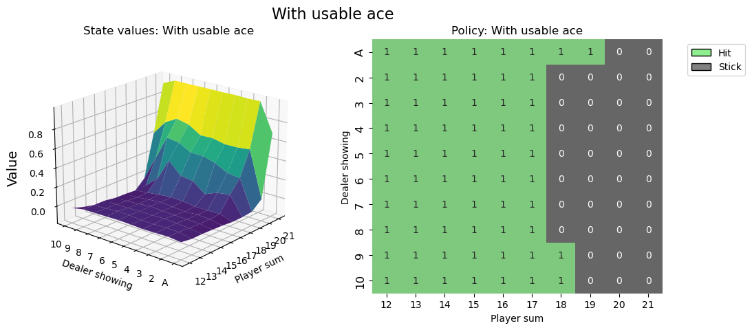
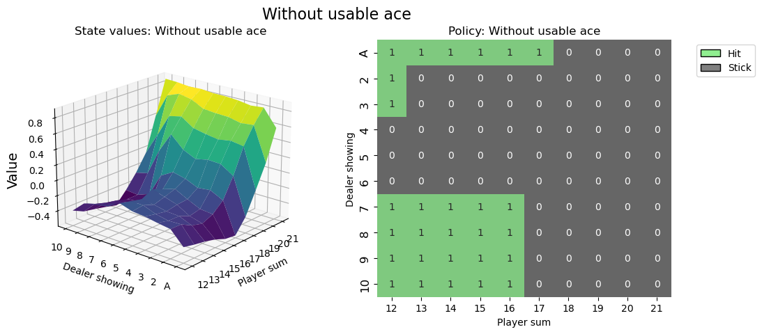
Visualizing the results
def create_grids(agent, usable_ace=False):

    # convert our state-action values to state values
    # and build a policy dictionary that maps observations to actions
    V = defaultdict(float)
    policy = defaultdict(int)
    for obs, action_values in agent.q_values.items():
        V[obs] = np.max(action_values)
        policy[obs] = np.argmax(action_values)

    X, Y = np.meshgrid(
        np.arange(12,22), # players count
        np.arange(1,11))  # dealers face-up card

    # create the value grid for plotting
    Z = np.apply_along_axis(
        lambda obs: V[(obs[0], obs[1], usable_ace)], axis=2, arr=np.dstack([X, Y])
        )
    value_grid = X, Y, Z

    # create the policy grid for plotting
    policy_grid = np.apply_along_axis(
        lambda obs: policy[(obs[0], obs[1], usable_ace)], axis=2, arr=np.dstack([X, Y])
        )
    return value_grid, policy_grid
def create_plots(value_grid, policy_grid, title='N/A'):

    # create a new figure with 2 subplots (left: state values, right: policy)
    X, Y, Z = value_grid
    fig = plt.figure(figsize=plt.figaspect(0.4))
    fig.suptitle(title, fontsize=16)

    # plot the state values
    ax1 = fig.add_subplot(1, 2, 1, projection='3d')
    ax1.plot_surface(X, Y, Z, rstride=1, cstride=1,
                    cmap='viridis', edgecolor='none')
    plt.xticks(range(12, 22), range(12, 22))
    plt.yticks(range(1,11), ['A'] + list(range(2,11)))
    ax1.set_title('State values: ' + title);
    ax1.set_xlabel("Player sum")
    ax1.set_ylabel("Dealer showing")
    ax1.zaxis.set_rotate_label(False)
    ax1.set_zlabel('$V_{\pi}$', fontsize=14, rotation=0)
    ax1.view_init(20, 220)

    # plot the policy
    a2x = fig.add_subplot(1, 2, 2)
    ax2 = sns.heatmap(policy_grid, linewidth=0, annot=True, cmap="Accent_r", cbar=False)
    ax2.set_title('Policy: ' + title);
    ax2.set_xlabel("Player sum")
    ax2.set_ylabel("Dealer showing")
    ax2.set_xticklabels(range(12, 22))
    ax2.set_yticklabels(['A'] + list(range(2,11)), fontsize=12)

    # add a legend
    legend_elements = [Patch(facecolor='lightgreen', edgecolor='black', label='Hit'),
                       Patch(facecolor='grey', edgecolor='black', label='Stick')]
    ax2.legend(handles=legend_elements, bbox_to_anchor=(1.3, 1))
    return fig
# state values & policy with usable ace (ace counts as 11)
value_grid, policy_grid = create_grids(agent, usable_ace=True)
fig1 = create_plots(value_grid, policy_grid, title='With usable ace')
plt.show()
# state values & policy without usable ace (ace counts as 1)
value_grid, policy_grid = create_grids(agent, usable_ace=False)
fig2 = create_plots(value_grid, policy_grid, title='Without usable ace')
plt.show()
It’s good practice to call env.close() at the end of your script, so that any used ressources by the environment will be closed.
env.close()
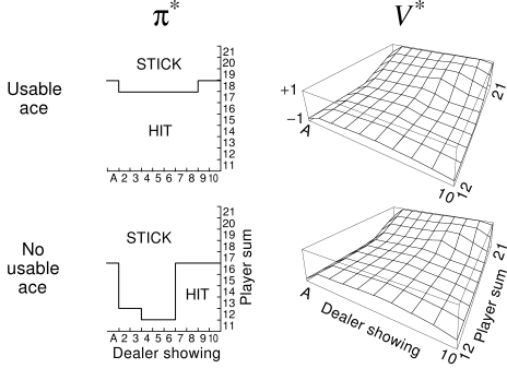
Optimal policy
For reference, here the optimal policy and value function, which we were able to achieve <:) (taken from Sutton & Barto):
I hope that this Tutorial helped you get a grip of how to interact with OpenAI-Gym environments and sets you on a journey to solve many more RL challenges.
It is recommended that you solve this environment by yourself (project
based learning is really effective!). You can apply your favorite
discrete RL algorithm or give Monte Carlo ES a try (covered in Sutton &
Barto, section
5.3) - this way you can compare your results directly to the book.
Best of fun!