Policy Evaluation and Value Iteration

Introduction
If we have a finite set of states, we can write the state values as a vector, where the entry at position $i$ corresponds to the state value $V^{\pi}_{s_i}$ of state $s_i$:
($n = |S|$ so that the formulas are easier to read). To see what’s going on, let’s write out the vectorized bellman equation for the state-values of policy $\pi$ and open them up:
\[\begin{align*} \tag{1}\label{eq:1} \boldsymbol{V}^{\pi} = \begin{bmatrix} V^{\pi}_{s_1} \\ V^{\pi}_{s_2} \\ \vdots \\ V^{\pi}_{s_n} \end{bmatrix} &= \boldsymbol{R}^{\pi} + \gamma \boldsymbol{P}^{\pi} \boldsymbol{V}^{\pi} \\ &= \begin{bmatrix} R^{\pi}_{s_1} \\ R^{\pi}_{s_2} \\ \vdots \\ R^{\pi}_{s_n} \end{bmatrix} + \gamma \begin{bmatrix} P^{\pi}_{s_1 s'_1} & P^{\pi}_{s_1 s'_2} & \dots\\ \vdots & \ddots & \\ P^{\pi}_{s_n s'_1} & & P^{\pi}_{s_n s'_n} \end{bmatrix} \begin{bmatrix} V^{\pi}_{s_1} \\ V^{\pi}_{s_2} \\ \vdots \\ V^{\pi}_{s_n} \end{bmatrix} &= \begin{bmatrix} R^{\pi}_{s_1} + \gamma \sum_{s'} P^{\pi}_{s_1 s'} V^{\pi}_{s'} \\ \vdots \\ R^{\pi}_{s_n} + \gamma \sum_{s'} P^{\pi}_{s_n s'} V^{\pi}_{s'} \\ \end{bmatrix} \end{align*}\]Analytic solution
To solve for $\boldsymbol{V}^{\pi}$ in equation \ref{eq:1}, we can first subtract $\gamma \boldsymbol{P}^{\pi} \boldsymbol{V}^{\pi}$ from both sides of the equation to get both $\boldsymbol{V}^{\pi}$ on one side:
\[\boldsymbol{V}^{\pi} - \gamma \boldsymbol{P}^{\pi} \boldsymbol{V}^{\pi} = \boldsymbol{R}^{\pi}\]Next, we can factor out $\boldsymbol{V}^{\pi}$ from the left-hand side to get
\[(\boldsymbol{I} - \gamma \boldsymbol{P}^{\pi}) \boldsymbol{V}^{\pi} = \boldsymbol{R}^{\pi}\]Note that for the factorization of $\boldsymbol{V}^{\pi}$, we don’t get $\boldsymbol{V}^{\pi} = 1 * \boldsymbol{V}^{\pi}$, but instead we need to use the identity matrix: $\boldsymbol{V}^{\pi} = \boldsymbol{I} \boldsymbol{V}^{\pi}$.
Finally, we can multiply with the inverse matrix of $(1 - \gamma \boldsymbol{P}^{\pi})$ to obtain the analytic fixed point (or equlibrium) of the true state values $\boldsymbol{V}^{\pi}$ for policy $\pi$:
\[\begin{equation} \tag{2}\label{eq:2} \boldsymbol{V}^{\pi} = (\boldsymbol{I} - \gamma \boldsymbol{P}^{\pi})^{-1} \boldsymbol{R}^{\pi} \end{equation}\]Policy evaluation
Policy evaluation algorithm:
Input: policy $\pi$
Output: approximated $V^{\pi}$
-
Initialize $V(s), V’(s)$ arbitrarily (e.g. to 0)
-
While True:
- $\Delta \leftarrow 0$ // maximum difference of a state-value
- For each $s \in S$:
- $V’(s) \leftarrow \sum_{a} \pi(s,a) \sum_{s’} P_{s,s’}^{a}[R_{s,s’}^{a} + \gamma V(s’)]$
- $\Delta \leftarrow$ max $(\Delta, \vert V’(s)-V(s)\vert)$
- $V(s) \leftarrow V’(s)$
- $V’(s) \leftarrow \sum_{a} \pi(s,a) \sum_{s’} P_{s,s’}^{a}[R_{s,s’}^{a} + \gamma V(s’)]$
- If $\Delta < \epsilon$:
- return approximated $V^{\pi}$
- $\Delta \leftarrow 0$ // maximum difference of a state-value
Value iteration
You can use the analytic solution \eqref{eq:2} to find the fixed point of $\boldsymbol{V}^\pi$ for MDPs with small state-spaces (working definition for this post: the problem is small iff the state-transition-probability matrix $\boldsymbol{P}^\pi$ with $|S|^2$ entries fits into main memory). If $|S|^2$ is too large though, so that it doesn’t fit into main memory (this will be the case for many MDPs that we encounter, and often times we deal with huge state spaces), we can find an approximate solution by performing value iteration. For the value iteration algorithm to work, the following criteria must be met:
- We need the transition probabilities $P^a_{ss’} = P(s’|s,a)$.
- The probabilitiy distribution $P(r|s,a,s’)$ for the random variable $R^a_{ss’}$ must also be available to us.
Value iteration algorithm:
Input: MDP with a finite number of states and actions
Output: approximated $V^{*}$
-
Initialize $V(s), V’(s)$ arbitrarily (e.g. to 0)
-
While True:
- $\Delta \leftarrow 0$ // maximum difference of a state-value
- For each $s \in S$:
- $V’(s) \leftarrow \max_{a} \sum_{s’}\sum_{r} P(s’,r | s,a) [r + \gamma V(s’)]$
- $\Delta \leftarrow$ max $(\Delta, \vert V’(s)-V(s)\vert)$
- $V(s) \leftarrow V’(s)$
- $V’(s) \leftarrow \max_{a} \sum_{s’}\sum_{r} P(s’,r | s,a) [r + \gamma V(s’)]$
- If $\Delta < \epsilon$:
- return approximated $V^{*}$.
- $\Delta \leftarrow 0$ // maximum difference of a state-value
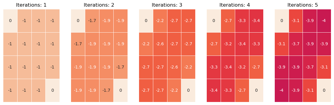
If we repeat this infinitely often, then the state values will converge to the true value function $V^{\pi}$:
\[\lim_{k \to \infty} \boldsymbol{V}^{k} = \boldsymbol{V}^{\pi}\]where $\boldsymbol{V}^{k}$ are the state-values in the $k$-th iteration.
To illustrate this, we can use this example MDP with a 4x4 grid as the state-space and two terminal states (upper left and bottom right cells). The action-space is $A=$ { $\text{left, right, up, down}$ } and each timestep that the agent is not in a terminal state, it receives a reward of -1.
Deriving an optimal policy:
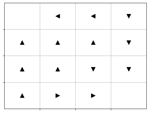
From the optimal state-value function $V^{*}$, it’s relatively simple to derive an optimal policy (there could always be multiple policies that are equally good).
\[\pi^{*}(s) = arg\max_{a} \sum_{s'}\sum_{r} P(s',r | s,a) [r + \gamma V(s')]\]An optimal policy for our gridworld-MDP would be:
- Note: You can do the book exercises and try to get a solution from Prof. Sutton here.
References
- Linear-algebra thumbnail from w3resource.com.
- Sutton & Barto: Reinforcement Learning
- Lemcke, J. Intelligent Data Analysis 2: Exercise-Notebook 6 (Rl)