Importance Sampling
Introduction
This blogpost describes the mathematical background for off-policy policy gradient methods.
Importance sampling is a statistics tool for estimating the expectation of a random variable that we can not sample from. It is applicable when the following preconditions are met:
- we can’t sample from the random variable of interest, maybe because it’s too expensive
(otherwise just sample from it) - but we know the probabilities of the individual values of this random variable
- we have a second random variabe that can take on the same values and that we can sample from.
This is especially useful in Reinforcement Learning if we already have some collected samples from an old policy and we want to update a new policy with them. The goal is to calculate the expectation of the new policy, and all the prerequisites are satisfied because for each collected experience, we can calculate the probability that the new policy would have taken that action.
With importance sampling, we can rewrite the expectation of the target random variable into an expectation with respect to the second random variable that we can sample from.
Using this trick, we can use offline Reinforcement Learning (replay buffers) for policy gradient methods!
Derivation
Definitions for expectations of a random variable $x$ with regard to a probability function $f$ (and in the second case $g$):
\[\begin{align*} \mathbb{E}_f [x] &\dot{=} \sum_x f(x) x \\ \mathbb{E}_g [x] &\dot{=} \sum_x g(x) x \end{align*}\]Rewriting the expectation with respect to another function (from target $g$ to sampling variable $f$):
\[\begin{align*} \mathbb{E}_g [x] &\dot{=} \sum_x g(x) x \\ &= \sum_x f(x) \frac{ g(x) }{ f(x) } x \;\; (\text{multiply with} \frac{f(x)}{f(x)}) \\ &= \mathbb{E}_f \left[ \frac{g(x) }{ f(x) } x \right] \\ \\ \end{align*}\]This results in the importance sampling formula.
\[\Rightarrow \mathbb{E}_f \left[ \frac{g(x) }{ f(x) } x \right] = \mathbb{E}_g \left[ x \right]\]Implementation
I used the example (the two dice with the given probabilities) from [2] so that I’m able to validate my results.
First we define our values, which are the face values of a normal 6-faced die.
import numpy as np

# values
x = np.arange(1,7) # 1-6
Then we define the probability functions $f$ and $g$.
# define f
f_probs = np.array([1 / len(x) for x_i in x]) # uniform (fair) distribution
print(f_probs)
# define g
g_probs = np.array([x_i / len(x) for x_i in x]) # biased (unfair) distribution
g_probs /= sum(g_probs)
print(g_probs)
Let’s start by approximating the mean of a fair die with $N=5000$ samples.
\[\mathbb{E}_f [x] \approx \frac{1}{N} \sum_{i=1}^{N} x_i\]N_samples = 5000
# get the samples using a pseudo-random generator
fair_die_samples = np.random.choice(x, size=N_samples, p=f_probs)
# calculate the mean of the samples for the fair die
approx_fair_die_mean = 1 / N_samples * np.sum(fair_die_samples)
# print the mean
print(f'approx_fair_die_mean: {approx_fair_die_mean:.3f}')
Now comes the importance sampling part to estimate $\mathbb{E}_g[x]$ by sampling from $f$.
\[\mathbb{E}_g \left[ x \right] = \mathbb{E}_f \left[ \frac{g(x) }{ f(x) } x \right] \approx \frac{1}{N} \sum_{i=1}^{N} \frac{g(x_i)}{f(x_i)} x_i \; \Big| \; x_i \sim f\]# calculate the mean of the samples for the biased die using importance sampling
approx_biased_die_mean = 0.0
for i in range(N_samples):
x_i = np.random.choice(x, p=f_probs)
approx_biased_die_mean += (g_probs[x_i-1] / f_probs[x_i-1]) * x_i
approx_biased_die_mean /= N_samples
# print the mean
print(f'approx_biased_die_mean: {approx_biased_die_mean:.3f}')
For reference, the theoretical expected values are:
\[\mathbb{E}_f [x] = 3.5 \\ \mathbb{E}_g [x] = 4.\bar{3}\]References
- Phil Winder, Ph.D. - Reinforcement Learning: Industrial Applications of Intelligent Agents
- Phil Winder - Importance Sampling Notebook
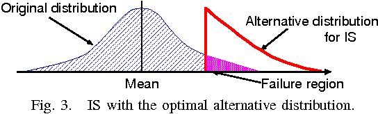
- Thumbnail taken from Sequential importance sampling for low-probability and high-dimensional SRAM yield analysis.