Gaussian processes and bayesian optimization
Contents
- Goal
- Gaussian Process
- Kernel function
- Covariance matrix
- Regression with the gaussian process
- Bayesian Optimization Algorithm
- Exploration and Exploitation
- Aquisition function: Expected Improvement
- Example for an Application
- Appendix: Statistical Basics (Variance, Covariance, Covariance matrix)
- References
Goal
In bayesian optimization, we want to optimize a target function $f$, which is costly to probe. A typical setting for this is hyperparameter optimization. Here, $f$ yields the empirical risk (average loss) of the model after training for a number of steps.
During the optimization, we try out differerent vectors of hyperparameters. To balance the exploration-exploitation tradeoff (exploration: pick a region with high variance; exploitation: pick a region where we expect a high reward), we need an aquisition function, which gives us the next hyperparameter vector $\lambda$.
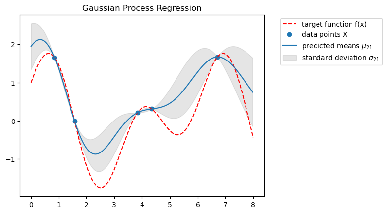
As input to our gaussian process, we are given a dataset $\mathcal{D}$ of probes, for example $\mathcal{D} = { (x_1, f(x_1)), (x_2, f(x_2)), (x_3, f(x_3)) }$. The task is to predict the mean $\mu_*$ for and variance $var_*$ for the function value $f(x_*)$ of a new input $x_*$.
To do that, we assume that it follows the same distribution as the dataset: $f(x_*) \sim \mathcal{N}(m(x_*), k(x_*, x_*))$
Gaussian Process
A gaussian process is a stochastic process that defines a stochastic value $y$ for every time step $t$. Therefore, it can be seen as a distribution over functions $f$ with $f(x) = y$. These functions are just vectors of function values $f(x)$ that can be sampled from the process.
To define a gaussian process $GP$, we need a mean function $m(x)$ and a kernel $k(x,x’)$ as a covariance function:
\[f(x) \sim GP( m(x), k(x,x') ).\]In the gaussian process, the mean and covariance are correlated with the other input data, as defined by the mean and covariance functions. This is more expressive than a simple multivariate gaussian, where the function values are jointly distributed and not correlated.
We use a kernel function to model the covariance of two data points. By picking a specific kernel function, we put prior information into the model (e.g. how smooth the function is).
Kernel function
In our gaussian process model, we assume that if two x values are close to each other, their corresponding y values with y=f(x) are also similar. Using this assumption, we can model the covariance (matrix) using a kernel function. This function has to be positive-definite, which means among other things that it has a global maximum at $x=0 \implies \forall x. f(0) \geq f(x)$. This property must be satisfied because the covariance of two identical x has to be maximal.
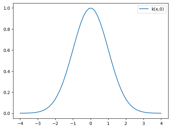
One popular choice for the kernel is to use a radial basis function (RBF), which looks like this:
\[k(x,x') = \exp(-\frac{1}{2 \sigma^2} ||x-x'||^2) = \begin{cases} 1 & \text{if } x=x' \\ \text{small } (\approx 0) & \text{if } x \text{ and } x' \text{ are far apart}\\ \end{cases}\]def kernel_fn(x1,x2):
""" RBF kernel function """
sigma = 1
return np.exp(-0.5 * sigma**2 * np.dot(x1-x2, x1-x2))
If we plot the RBF kernel function for a scalar variable x as the first argument and 0 as the second argument, we observe that it indeed has a global maximum at $x=0$ ($\rightarrow$ positive-definite ✅) and it drops off towards 0 as the x values get further apart.
Covariance matrix
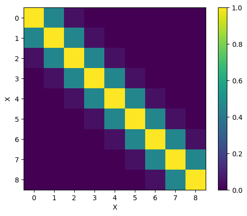
Using our kernel function, we can model (predict) the Covariance matrix $\Sigma$:
\[\Sigma = \mathbb{E}[ (X-\mu_X) (Y-\mu_Y)^T ] \; \text{ with } \; \Sigma_{ij} = cov(X_i, Y_i)\]With the RBF kernel, the visualized $9 \times 9$ covariance matrix $\Sigma$ looks like this:
We can also use a finer matrix ($200 \times 200$) to get a smooth view at what the function does:
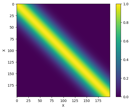
Just notice that for the two covariance matrices above, the kernel yields higher values (up to 1) for $x$ values that are close to each other.
Regression with the gaussian process
We use the $GP$ (which includes some assumptions in our kernel choice) as a prior and create a posterior distribution using our data. Using the posterior, we can predict the mean and variance of function values $\mathbf{y}_2$ for new data samples $X_2$.
Solution
Mean of $\mathbf{y}_2$:
\[\mu_{2|1} = (\Sigma_{11}^{-1} \Sigma_{12})^T \mathbf{y}_1\]Variance of $\mathbf{y}_2$:
\[\Sigma_{2|1} = \Sigma_{22} - (\Sigma_{11}^{-1} \Sigma_{12})^{\top} \Sigma_{12} \\\]Bayesian Optimization Algorithm
used_parameters = dict()

# maybe give it N hours to train and update the budget using wallclock time
budget = 10

while budget:
    hyperparam_vector = argmax(expected_improvement(GP))

    # train and evaluate model with the picked hyperparameters
    y = f(hyperparam_vector)

    used_parameters[hyperparam_vector] = y
    budget = budget - 1

# return hyperparam_vector with the minimal loss in f
- Draw a vector $f$ (which is basically a function if the vector has infinite length):
- Get the loss, which is stochastic (depends on SGD etc.):
Exploration and Exploitation
Exploration: Prefers values that have a high posterior variance
(where we don’t know much about the outcome yet).
Exploitation: Prefers values where the posterior has a high mean $\mu_x$.
Aquisition function: Expected Improvement
To balance the exploration-exploitation tradeoff, we need an aquisition function that tells us which hyperparameter-vector $\lambda$ to pick next from the values in $X2$ when the data $X1, y1$ is given.
One possible aquisition function is Expected Improvement (EI):
\[A(\lambda \in X2 | X1,y1) = \mathbb{E}[ \max(0, y_{\max}) - y ] = \begin{cases} (\mu - y_{\max} - a) \cdot CDF(Z) + \sigma \cdot PDF(Z) & \text{if}\ \sigma > 0 \\ 0 & \text{if}\ \sigma = 0 \end{cases}\]with
\[Z = \begin{cases} \frac{\mu - y_{\max} - a}{\sigma} &\text{if}\ \sigma > 0 \\ 0 & \text{if}\ \sigma = 0 \end{cases}\]and the hyperparameter $a$ for exploration (higher $a$ means more exploration).
A common default value is $a = 0.01$ [7].
Example for an Application
Bayesian optimization was used for hyperparameter tuning in the AlphaGo system, more details can be found in the dedicated paper.
Appendix: Statistical Basics (Variance, Covariance, Covariance matrix)
Variance (scale by N-1 for a population):
\[var(x) = \frac{1}{N} \sum_{i=1}^{N} (X_i - \mu_X)^2\]Covariance (scale by N-1 for a population):
\[cov(X,Y) = \frac{1}{N} \sum_{i=1}^{N} (X_i - \mu_X) (Y_i - \mu_Y)\]If you plug in X two times into the covariance formula, notice that $cov(X,X) = var(X)$.
References
- Thumbnail: Gaussian process regression (sklearn docs)
- Baysian Optimization - Implementation for Hyperparameter Tuning (GitHub Repo)
- Nando de Freitas: Machine learning - Introduction to Gaussian processes
- Cornell: Lecture 15: Gaussian Processes (well written notes)
- Gaussianprocess Notes (includes implementation)
- Peter Roelants’s blog: Gaussian processes (1/3) - From scratch
- Martin Krasser’s blog: Bayesian optimization (includes Expected Improvement formula)