Transformers

First draft: 2023-02-20
Introduction
The Transformer was introduced in the “Attention is all you need” paper in 2017 and has held the state of the art title in Natural Language Processing for the last 5-6 years. It can be applied to any kind of sequential task and is successful in a lot of domains and with many variations (although the architecture presented in the 2017 paper still pretty much still applies today).
The basic idea of the Transformer is to build an architecture around attention-functions. Multiplicative attention blocks (where the weighting factors of the values are calculated by a dot-product between queries and keys) can be parallelized and become super fast. This is one of the major advantages over all types of RNNs, where the input has to be processed sequentially. Another advantage is the number of processing steps between inputs that are multiple timesteps apart: for RNNs capturing long-range dependencies is really difficult and with Transformers, the inputs are related in a constant number of processing steps and theirfore even long-range dependencies can be captured pretty easily using attention.
Goal of this blogpost
The goal for this post is to build a encoder-only transformer. The left side of the transformer in the picture is the encoder, which you would use for tasks that require additional information that first needs to be encoded, an example would be a translation task, where you first have to encode the sentence in the original language using the encoder. Then you can use the decoder to process the growing sequence of tokens in the target language.
We’ll only use the encoder part with self-attention, because we just want to have a text-block as context (prompt) and complete it (meaning we can generate more text that fits the given prompt) and theirfore don’t need both parts.
Architecture
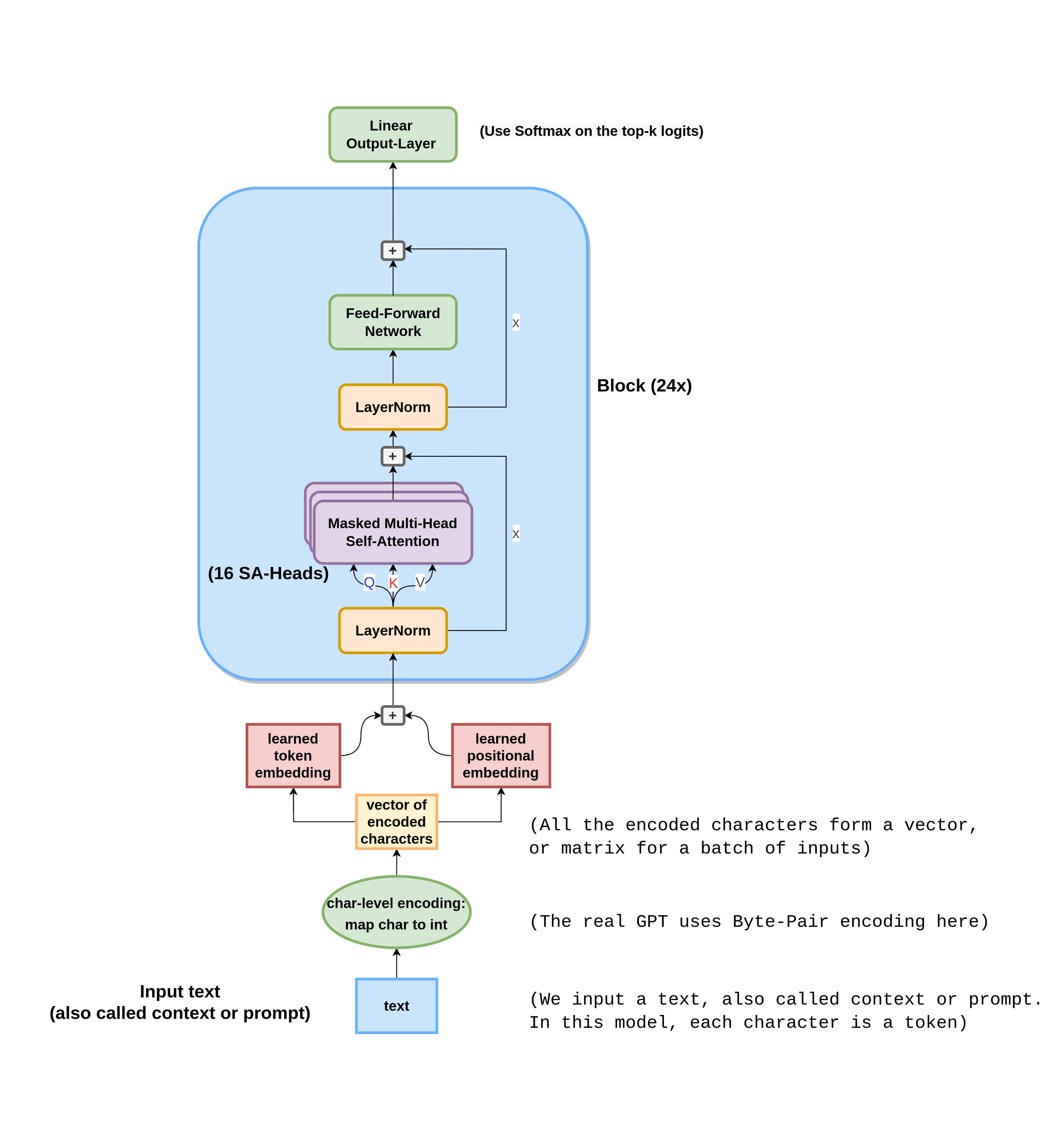
For reference how each part that we’ll talk about is integrated, here is a complete view of the encoder-only transformer architecture:
Encodings
Character-level Encoding
Character-encoding just maps every unique character in the text corpus to an integer. With punctuation, digits, letters (including some chinese I believe) the Lex Fridman podcast turns out to include around 150 unique characters. As you probably can imagine, this is the easiest form of tokenization to implement.
Byte-Pair Encoding (BPE)
BPE is used very commonly in practice, for example for the GPT models by OpenAI. It is a form of sub-word tokenization and combines the advantages of giving the model easier access to common sub-words (the byte pairs), which should make it easier to generate comprehensive language, as well as the ability to also understand uncommon words more intuitively through their sub-words (as you can split them into their prefixes, suffixes etc., which should be more common than the combined word).
Here are the 150 (approximately) most common byte pairs from my dataset:
Embeddings
Token embedding
Every token has a learned embedding in the token embedding table.
Positional embedding
The position is embedded using a learned second embedding table. The token-embedding and position-embedding matrices are added to get the input for the transformer.
Attention
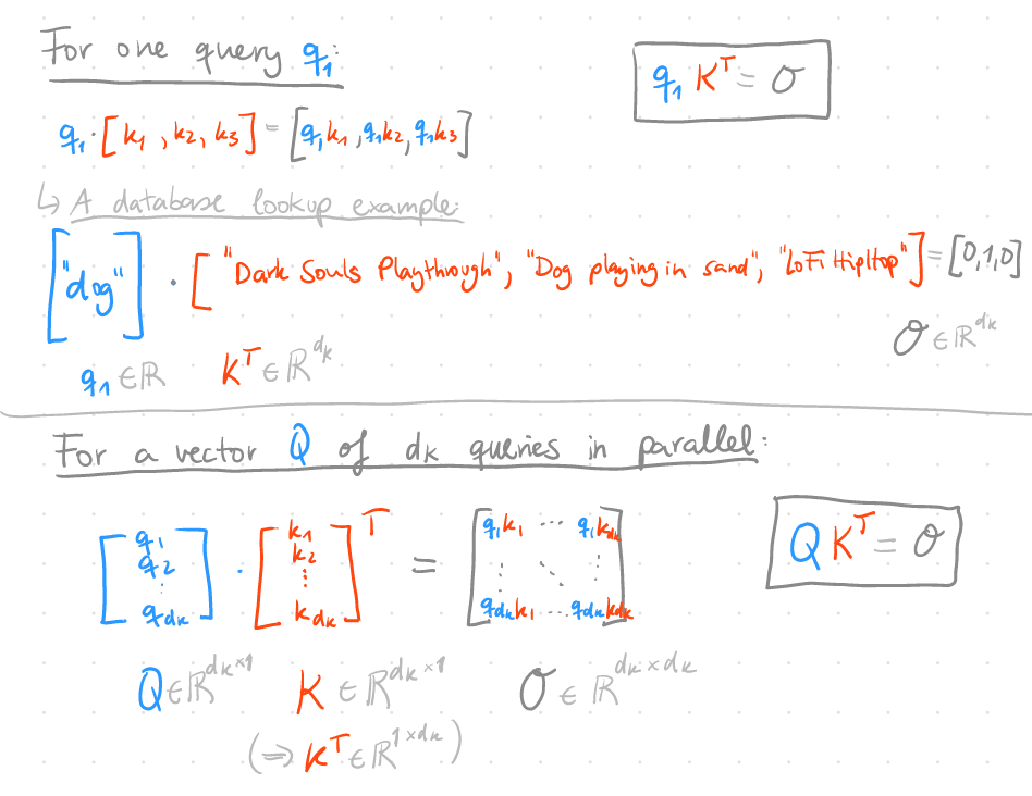
I find attention very intuitive to understand when you look at it from a database perspective: You have your query (Q), key (K) and value (V) vectors and want to weight the values according to how much a query matches with every value. If you have a database lookup with one hit, the query-key pair for the hit would result in a weight of 1 and every other query-key pair would result in a weight equal to 0, so only the value for that matching key gets returned.
We use vector products to do this weighting, and thus can have more than one query. Actually we can process a vector Q of queries that gets matched against keys to create a weight matrix where row $i$ corresponds to the weights for the corresponding query $q_i$.
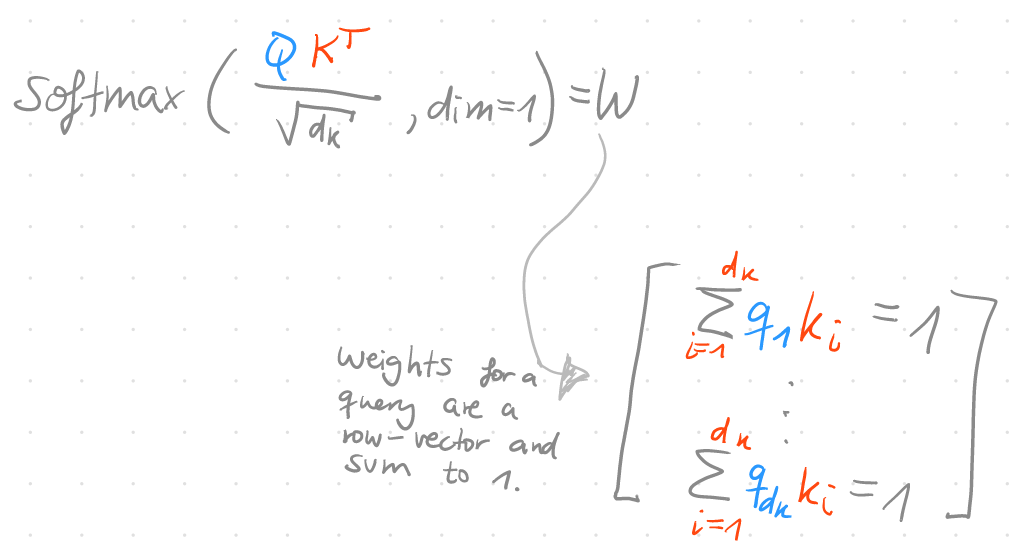
Scaling
Actually this is not enough to get proper weighting factors, because the weights should sum to 1. To achieve this, we can apply a softmax per row (dim=1). In the “Attention is all you need” paper, they also scale the matrix by a factor of $\frac{1}{\sqrt{d_k}}$. If you don’t do that, the gradient for large arguments of the softmax function is tiny and theirfore the entire architecture doesn’t learn as quickly without scaling.
The gradient of the softmax function is:
To illustrate the difference that scaling the weight-logits has on the gradient, I took the gradient $\frac{\partial z}{\partial z_0}$ of the vector $z = [z_0, z_1, z_2, z_3] = [1, 20, 3, 4]$. The resulting gradient is already tiny with just one larger number (the 20 at index 1):
Tiny gradient without scaling:
Here $d_k = 4$, so we multiply the matrix $X$ by the scaling factor $\frac{1}{\sqrt{4}}$ to get the scaled $X$. If we take the gradient now, it’s not as small as the previous gradient. This way our network can learn quicker.
Better gradient via scaling:
The resulting weight matrix W can finally be multiplied with the value vector V to get the output of one (scaled dot-product) attention unit:
\[\text{Attention}(Q,K,V) = WV = \text{softmax}(\frac{QK^T}{\sqrt{d_k}})V\]Implementing Attention
First, let’s create some random vectors for Q, K and V with shape $5 \times 1$.
Q = torch.rand(5,1)
K = torch.rand(5,1)
V = torch.rand(5,1)
We get the logits for the weight matrix by using the scaled query-key matrix multiplication. In PyTorch, we can use the @-Symbol to perform a matrix multiplication.
C, B = Q.shape # Channels and Batch-Size

W = (Q @ K.T) / torch.sqrt(torch.tensor(C))
W
[0.0539, 0.2369, 0.0690, 0.1660, 0.1998],
[0.0256, 0.1125, 0.0328, 0.0788, 0.0949],
[0.0198, 0.0870, 0.0254, 0.0610, 0.0734],
[0.0781, 0.3433, 0.1000, 0.2405, 0.2895],
[0.0246, 0.1081, 0.0315, 0.0757, 0.0912]])
To get the final weight matrix, we apply a softmax on each row. Each row now sums up to 1.
W = F.softmax(W, dim=1)
W
[0.1964, 0.2037, 0.1970, 0.2007, 0.2021],
[0.1983, 0.2018, 0.1986, 0.2004, 0.2010],
[0.1987, 0.2014, 0.1989, 0.2003, 0.2008],
[0.1949, 0.2055, 0.1956, 0.2010, 0.2030],
[0.1984, 0.2017, 0.1986, 0.2004, 0.2010]])
Now we just have to apply our computed weight-matrix to our values to get the final attention output.
W @ V
[0.4725],
[0.4733],
[0.4734],
[0.4719],
[0.4733]])
Concise Implementation of Scaled Dot-Product Attention
Putting it all together, we get:
def attention(Q,K,V):
    """
    Applies scaled dot-product attention
    between vectors of queries Q, keys K and values V.
    """
    d_k = torch.tensor(Q.shape[0])
    W =  F.softmax((Q @ K.T) / torch.sqrt(d_k), dim=1)
    return W @ V
In our actual implementation we use the attention head as a class which also already includes the linear projections for the query, key and value vectors:
class SelfAttentionHead(nn.Module):

    def __init__(self):
        super().__init__()
        self.proj_q = nn.Linear(embed_dims, head_size, bias=False)
        self.proj_k = nn.Linear(embed_dims, head_size, bias=False)
        self.proj_v = nn.Linear(embed_dims, head_size, bias=False)
        self.dropout = nn.Dropout(dropout)

    def forward(self, x):
        """
        Applies masked scaled dot-product attention
        between vectors of queries Q, keys K and values V.
        """
        B,T,C = x.shape

        Q = self.proj_q(x)
        K = self.proj_k(x)
        V = self.proj_v(x)

        W = (Q @ K.transpose(-1,-2)) # (B, T, C) @ (B, C, T) ==> (B,T,T)
        W /= torch.sqrt(torch.tensor(head_size))

        # mask out forbidden connections
        tril = torch.tril(torch.ones((block_size, block_size), device=device))
        W = W.masked_fill(tril[:T, :T]==0, float("-inf")) # make smaller so it fits if context < block_size
        W = F.softmax(W, dim=1)
        W = self.dropout(W)

        out = W @ V
        return out # (B,T,C=head_size)
Masking
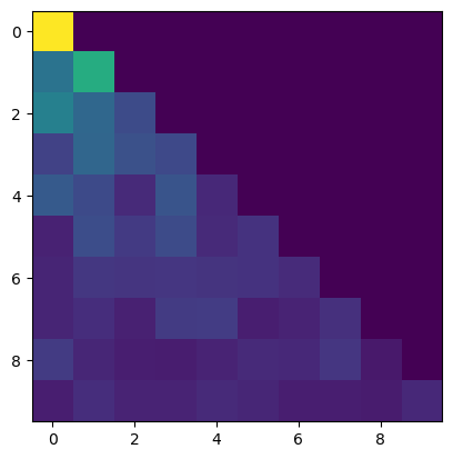
Notice that a self-attention head masks its inputs.
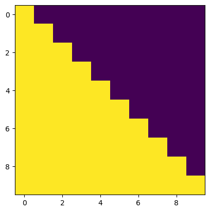
We want a position to only attent to the past in the decoder block, because they won’t have future tokens available yet and thus can’t learn to attent to the future. Each token can only attent to it’s own position and all past positions in the given context sequence. To mask all attention connections to the future out, we use a lower triangular matrix (note: tril means triangular-lower).
T = 10
tril = torch.tril(torch.ones((T,T)))
plt.imshow(tril)
W = torch.rand((T,T)) # there will be real data here

# mask out forbidden connections
W = W.masked_fill(tril==0, float("-inf")) # set everywhere where tril is 0 to -inf (upper right)

W = F.softmax(W, dim=-1)
plt.imshow(W)
Multi-Head Attention
Linear Projection
In multi-headed attention, we apply multiple attention blocks in parallel. To encourage that they learn different concepts, we first apply linear transformation matrices to the Q, K, V vectors. You can intuitively look at this as viewing the information (vectors) from a different angle.
To get an idea about how this looks, here is a simple linear transformation of the unit vector $v = \begin{bmatrix} 1 \ 1 \end{bmatrix}$ in 2D space.
|
$$
A = \begin{bmatrix} -0.7 & 1 \\ 1 & -0.2 \end{bmatrix} \\
$$
|
$$
v = \begin{bmatrix} 1 \\ 1 \end{bmatrix} \\
$$
|
$$
Av = \begin{bmatrix} 0.3 \\ 0.8 \end{bmatrix}\\
$$
|
|---|
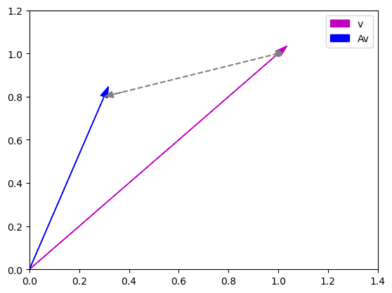
We can simply implement these linear projections as a Dense layer without any biases. The weights of the projections can be learned so that the Transformer uses the most useful projections of the Q,K,V vectors. A useful property of these projections is that we can pick the number of dimensions for the space that they are projected into, which usually has a lower dimensionality than the input vectors so that it is computationally feasible to have multiple heads running in parallel (you want to set it so that your GPUs VRAM is maximally utilized).
To implement multi-head attention, we first define linear layers for each head and for each Q,K,V vector. We also need a linear layer that combines the output of all parallel attention blocks into one output vector.
class MultiHeadAttention(nn.Module):

    def __init__(self):
        super().__init__()

        self.heads = nn.ModuleList([SelfAttentionHead() for i in range(n_heads)])
        self.proj = nn.Linear(embed_dims, embed_dims, bias=False) # embed_dims = n_heads * head_size
        self.dropout = nn.Dropout(dropout)

    def forward(self, x):

        out = torch.cat([attn_head(x) for attn_head in self.heads], dim=-1)
        out = self.dropout(self.proj(out))
        return out
Add & Norm and Residual Connections
We use pre-layernorm (performs bettern than post-layernorm), which is different from the original transformer. What we keep is the residual connections around the multi-head self-attention and around the mlp (simple feed-forward network with 2 dense layers and relu activations).
A transformer block also includes a feed forward network, so that it follows these two stages:
- Communicate via self-attention
- Process the results using the MLP
class Block(nn.Module):

    def __init__(self):
        super().__init__()
        self.attn = MultiHeadAttention()
        self.ln1 = nn.LayerNorm(embed_dims)
        self.ln2 = nn.LayerNorm(embed_dims)

        self.mlp = nn.Sequential(
            nn.Linear(embed_dims, 4*embed_dims), # following attention-is-all-you-need paper for num hidden units
            nn.ReLU(),
            nn.Linear(4*embed_dims, embed_dims),
            nn.Dropout(dropout),
        )

    def forward(self, x):

        # Applies layernorm before self-attention.
        # In the attention-is-all-you-need paper they apply it afterwards,
        # but apparently pre-ln performs better. pre-ln paper: https://arxiv.org/pdf/2002.04745.pdf

        x = x + self.attn(self.ln1(x)) # (B,embed_dims)
        x = x + self.mlp(self.ln2(x))
        return x
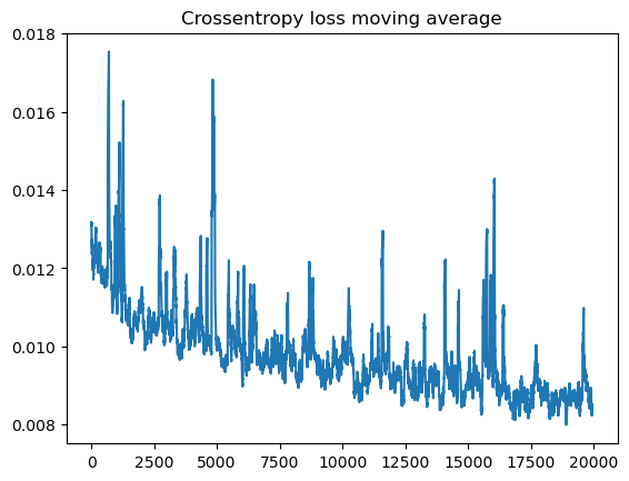
Training
References
- Thumbnail
- Transformer architecture image.
- Vaswani et. al: Attention Is All You Need - Paper
- Rasa: Rasa Algorithm Whiteboard - Transformers & Attention 1: Self Attention (This is the first video of a 4-video series about the Transformer, I can highly recommend it!)
- Andrej Karpathy: Let’s build GPT: from scratch, in code, spelled out. (Implementation)
- harvardnlp - The Annotated Transformer
- Aleksa Gordić: Attention // <- this is part 1
- Aleksa Gordić: Transformer // <- and part 2
- 11-785 Deep Learning Recitation 11: Transformers Part 1 (Implementation)
- TensorFlow Blog: A Transformer Chatbot Tutorial with TensorFlow 2.0
- Kaduri’s blog: From N-grams to CodeX (Part 2-NMT, Attention, Transformer)
- AI Coffee Break with Letitia: Positional embeddings in transformers EXPLAINED - Demystifying positional encodings.
- Ruibin Xiong et. al: On Layer Normalization in the Transformer Architecture (Pre-LayerNorm paper)