Actor Critics

First draft: 2022-10-24
Second draft: 2022-12-12
Third draft: 2022-12-15
Implementation: 2022-12-20
GAE: 2022-12-30
Dopaminergic circuit in our brain: 2022-12-31

If you are looking for code ...

I also wrote a tutorial implementing the theory presented in this blogpost for the gymnasium docs. The tutorial shows the implementation of an Advantage Actor-Critic (A2C) and also includes some notes on performance analysis, vectorized environments and domain randomization. You can find it here.

Introduction

The Actor Critic is a powerful and beautiful method of learning, with surprising similarities to our dopaminergic learning circuits.

Let’s start by looking at the REINFORCE algorithm, a method for training reinforcement learning (RL) agents. It is a policy gradient method, which means that it uses gradient ascent to adjust the parameters of the policy in order to maximize the expected reward. It does this by computing the gradient of the performance (goal) $\mathcal{J}(\theta) \stackrel{.}{=} V^{\pi_\theta}(s_0)$ with respect to the policy parameters, and then updating the policy in the direction of this gradient. This update rule is known as the policy gradient update rule, and it ensures that the policy is always moving in the direction that will increase the expected future reward (=return). Because we need the entire return $G_t$ for the update at timestep $t$, REINFORCE is a Monte-Carlo method and theirfore only well-defined for episodic cases.

One drawback of the pure REINFORCE algorithm is that it has a really high variance and could be unstable as a result. To lower the variance, we can substract a baseline $b(S_t)$, which has to be independent of the action. A good idea is to use state-values as a baseline, which reduce the magnitude of the expected reward (it has the effect of “shrinking” the estimated rewards towards the baseline value). Reducing the magnitude of the estimated rewards can help to reduce the variance of the algorithm. This is because the updates that the algorithm makes to the policy are based on the estimated rewards. If the magnitude of the rewards is large, the updates will also be large, which can cause the learning process to be unstable and can result in high variance. By reducing the magnitude of the rewards, the updates are also reduced, which can help to reduce the variance and thus stabilize the learning process.

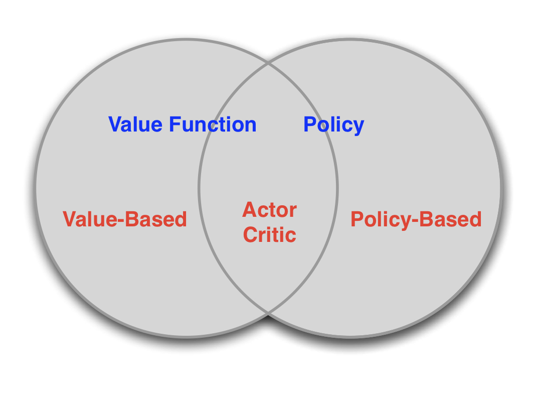
The Actor-Critic algorithm is an extension of the REINFORCE algorithm that uses a value function as a baseline to improve the stability of the learning process. This baseline also needs to be learned (we have to approximate $V(s)$, usually using a Deep Neural Network), theirfore Actor-Critics are a combination of value-based and policy-based methods:

Venn diagram taken from: David Silver, Lecture 7: Policy Gradient

From the Policy-Gradient-Theorem to Vanilla Policy Gradient (also called ‘REINFORCE’)

The policy gradient theorem (for the episodic case) states that:

\[\begin{align*} \nabla \mathcal{J}(\theta) &\propto \sum_s \mu(s) \sum_a Q^\pi(s,a) \nabla \pi(a|s,\theta) \\ &= \mathbb{E_\pi}[ \sum_a Q^\pi(s,a) \nabla \pi(a|s,\theta) ] \end{align*}\]

where $\mu(s)$ is the on-policy distribution over all states (included in $\mathbb{E}_\pi$). (From S&B [6], Chapter 13).
As a sidenote, $a(x) \propto b(x)$ states that a is proportional to b, meaning $a(x) = c \cdot b(x)$. This notation is sometimes useful for talking about gradients, because the factor $c$ is absorbed in the learning rate anyway.

We can extend the formula further by multiplying and deviding by $\pi(a|S_t, \theta)$ to get the expression $\frac{\nabla \pi(a|S_t, \theta)}{\pi(a|S_t, \theta)}$. This is a common trick using the logarithm, where you can rewrite the gradient of $\log x$ with $\nabla \log x = \frac{1}{x} \nabla x = \frac{\nabla x}{x}$ (just using the chain rule). In our specific case, we can use this as $\nabla \log \pi(a|S_t, \theta)$ $=$ $\frac{\nabla \pi(a|S_t, \theta)}{\pi(a|S_t, \theta)}$.

Performing all of the steps above:

\[\nabla \mathcal{J}(\theta) \propto \mathbb{E_\pi}[ \sum_a Q^\pi(s,a) \nabla \pi(a|s,\theta)]\] $ = \mathbb{E_\pi}[ \sum_a $ $\pi(a|S_t, \theta)$ $Q^\pi(s,a)$ $\frac{\nabla \pi(a|S_t, \theta)}{\pi(a|S_t, \theta)}$$]$

We can just replace $ \sum_a $ $\pi(a|S_t, \theta)$ $= 1$ and use the log-trick (rewrite the gradient of $\log x$ as the fraction described in the section above).

$ = \mathbb{E_\pi}[Q^\pi(s,a) $ $\nabla \log \pi(a|S_t, \theta)$$]$

$ = \mathbb{E_\pi}[G_t $ $\nabla \log \pi(a|S_t, \theta)$$]$

Temporal Difference (TD) Error

We can calculate the TD error as the difference between the new and old estimates of a state value:

\[\delta = r + \gamma V(s') - V(s)\]

The TD-Error denotes how good or bad an action-value is compared to the average action-value and thus is an unbiased estimate of the advantage $A(s,a)$ of an action. This is helpful if we want to update our network after every transition, because we can just use use the TD-Error in the place of the advantage to approximate it. Proof that the TD-Error approximates the advantage:

\[\begin{align*} \mathbb{E}[\delta^\pi|s,a] &= \mathbb{E}_\pi[G|s,a] - V^\pi(s,a) \\ &= Q^\pi(s,a) - V^\pi(s,a) \\ &= A^\pi(s,a) \end{align*}\]

Actor and Critic as Deep Neural Networks

The main idea is that we update the actor parameters in the direction of a value that is estimated by the critic, e.g. the advantage. This makes sense because the critic is better able to evaluate the actual value of a state.

As already mentioned, the actor is responsible for learning a policy $\pi(a|s)$, which is a function that determines the next action to take in a given state. The critic, on the other hand, is responsible for learning a value function $V(s)$ or $Q(s,a)$, which estimates the future rewards that can be obtained by following the policy. The actor and critic work together to improve the policy and value function over time, with the goal of maximizing the overall rewards obtained by the system.

Note, that it is common to use a shared neural network body. This is practical for learning features only once and not individually for both networks. The last layer of the body network connected to both the policy head and the value head), producing the outputs for actor and critic, respectively.

Actor Critic Algorithm

The following algorithm for an Actor Critic in the episodic case, we are calculating the TD-Error as $\delta \leftarrow R + \gamma \hat{V}(S’,w) - \hat{V}(S,w)$, using our parameterized state-value function (the critic). This means that all bootstrappinging of the TD-Error depends on our current set of parameters, which can introduce a bias. Theirfore, the updates only include a part of the true gradient. These methods are called semi-gradient methods.

Actor Critic algorithm (episodic):

Input: policy parameterization $\pi(a|s,\theta)$ (e.g. a Deep Neural Network),
state-value function parameterization $\hat{V}(s,\textbf{w})$ (e.g. a Deep Neural Network),

Parameters: learning rates for the actor: $\alpha_\theta$, and for the critic: $\alpha_\textbf{w}$
discount-factor $\gamma$

Initialize the parameters in $\theta$ and $\textbf{w}$ arbitrarily (e.g. to 0)
While True:
1. $S \leftarrow \text{env.reset()}$ // random state from starting distribution
2. $t \leftarrow 0$
3. While S is not terminal:
  1. $A \sim \pi(\cdot|S,\theta)$
  2. $S’, R \leftarrow \text{env.step}(A)$
  3. $\delta \leftarrow R + \gamma \hat{V}(S’,w) - \hat{V}(S,w)$
  4. $\textbf{w} = \textbf{w} + \alpha_\textbf{w} \delta \nabla_\textbf{w} \hat{V}(S,\textbf{w})$ // update critic
  5. $\theta = \theta + \alpha_\theta \gamma^t \delta \nabla_\theta \log \pi(A|S,\theta)$ // update actor
  6. $t \leftarrow t + 1$
  7. $S \leftarrow S’$

Output: parameters for actor: $\theta$, and critic: $\textbf{w}$

this implementation uses $\delta$ as an Advantage estimate (high variance)
$\delta$ can be replaced by one of the variations discussed in the sections above
pseudocode modified from Sutton&Barto [6], Chapter 13
great Stackexchange post for why we are using decay in the update of the actors parameters $\theta$.
Actor Critics work with discrete and continuous action spaces!

Variations

1) If we want to have no bias at all, we can calculate the advantage as the return $G_t \stackrel{.}{=} R_{t+1} + \gamma R_{t+2} + \gamma^2 R_{t+3} + \dots = \sum_{k=t+1}^{\infty} \gamma^k R_{t+k+1}$ minus the state-value. For this variation of the actor-critic algorithm, we can only do updates after each episode (because we need to calculate the return $G_t$).

\[\begin{align*} A(s,a) &= Q(s,a) - V(s) \\ &= r + \gamma V(s') - V(s) \\ &= G_t - V(s) \end{align*}\]

2) If you want to have less variance, you should use the actual returns (we have access to the entire reward list of an episode after letting it play out), but only for a couple of steps, and then after the k-th step use a state-value estimate produced by the critic network (this estimate is like an average of the previously seen returns from that state, so it will have less variance), but it will have a bias. We’ll discuss this tradeoff and solutions for it in the next section.

Overview of the Actor-Critic variations:

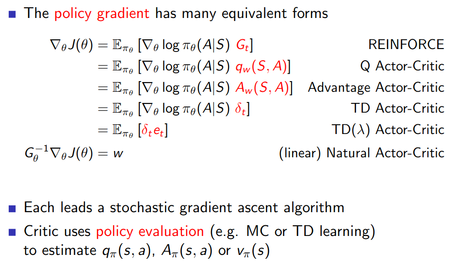
The most popular variation is the advantage actor critic (A2C).

Discrete versus Continuous

A great feature of policy-gradient methods is that they can be used for continuous action spaces. -> Soft Actor Critic (TODO)

Variance vs. Bias tradeoff for k-step returns

When estimating $Q(s,a)$ with semi-gradient methods (semi-gradient, because Function Approximation introduces a bias), we have to trade of bias and variance. We can either use our observed rollout to calculate $Q(s,a)$, or use our state-value-function $V(s)$ (=our critic Neural Network):

\[\begin{align*} \hat{Q}(s_t,a_t) &= \mathbb{E}[ r_{t+1} + \gamma r_{t+2} + \gamma^2 r_{t+3} + \dots ] \;\; (\text{ entire rollout}) \\ &= \mathbb{E}[ r_{t+1} + \gamma V(s_{t+1}) ] \;\; (\text{ short rollout}) \\ &= \mathbb{E}[ r_{t+1} + \gamma r_{t+2} + \dots + \gamma^k V(s_{t+k}) ] \;\; (\text{ k-step rollout}) \\ \end{align*}\]

For shorter k-step rollouts:

lower variance because the estimated state-value $\hat{V}(s)$ is an estimate based on lots of experience (=estimated average return).
higher bias, because the estimate is produced by the Neural Net

For longer k-step rollouts:

higher variance, because the return is only one observed monte-carlo rollout
low bias, because we use the actual return (no bias if we use the complete rollout)

Generalized Advantage Estimation (GAE)

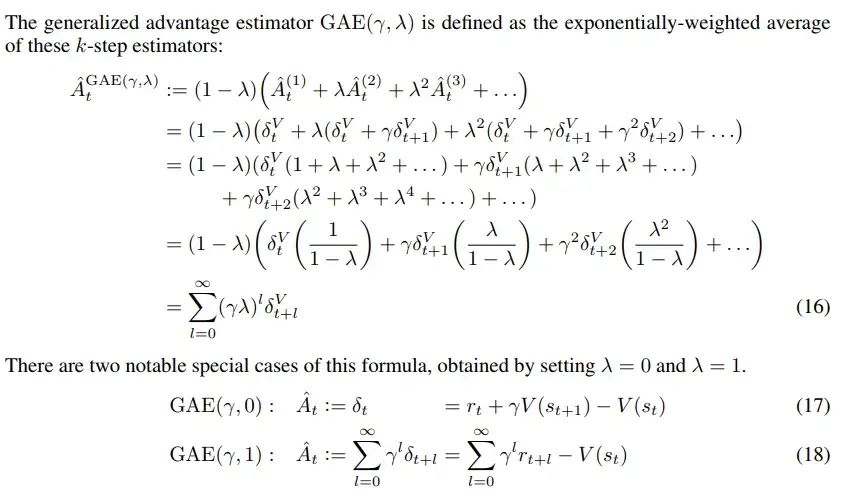
Generalized Advantage Estimation (GAE) is a method for estimating the advantages. It is an extension of the standard advantage function, which is calculated as the difference between the expected return of an action and the expected return of the current state. GAE uses a discount factor (lambda) to weight the different k-step rollouts for estimating Q.

By weighting the different k-step rollouts, we try to optimize the variance vs. bias tradeoff without having to search for a good hyperparameter k (the length of the rollouts). Again, we assume that the influence of an action decreases exponentially with a parameter $\lambda \in [0,1]$ over time (be careful with this assumption, depending on the environment!). The idea is pretty much the exact same as in TD($\lambda$).

see my TD($\lambda$) post or this blogpost about GAE by Jonathan Hui for more details.

From the GAE paper:

Calculating Q(s,a)-returns normally

for info, the ep_rewards and ep_value_preds tensors look like this (for one environment):
ep_rewards = [$r_1, \dots$]
ep_value_preds = [$V(s_0), \dots$]
(for multiple envs, $r_1$ would be a row with n_envs entries $\rightarrow$ shape=[n_steps_per_update, n_envs])
hyperparameters used: gamma=0.999

T = len(ep_rewards)
returns = torch.zeros(T, n_envs, device=device)
future_returns = torch.zeros(n_envs, device=device)

# compute the returns
for t in reversed(range(T)):
    future_returns = ep_rewards[t] + gamma * masks[t] * future_returns
    returns[t] = future_returns

print(returns.shape) # torch.Size([256, 3])

Calculating Q(s,a)-returns using GAE

hyperparameters used: gamma=0.999 and lam=0.9

T = len(ep_rewards)
returns = torch.zeros(T, n_envs, device=device)

# compute the returns using GAE ("Generalized Advantage Estimation" paper: https://arxiv.org/abs/1506.02438)
gae = 0.0
for t in reversed(range(T-1)):
    td_error = ep_rewards[t] + gamma * masks[t] * ep_value_preds[t+1] - ep_value_preds[t]
    gae = td_error + gamma * lam * masks[t] * gae
    returns[t] = ep_value_preds[t] + gae # Q(s,a) = V(s) + A(s,a)

print(returns.shape) # torch.Size([256, 3])

Here we are calculating the returns by using the following decomposition for the Q-values:

\[Q(s,a) = V(s) + A(s,a)\]

You can also leave out adding ep_value_preds[t] at the end and just save your generalized advantage estimates (gae) in an advantages tensor: advantages[t] = gae.

Async Advantage Actor Critic (A3C)

Picture taken from this blogpost.

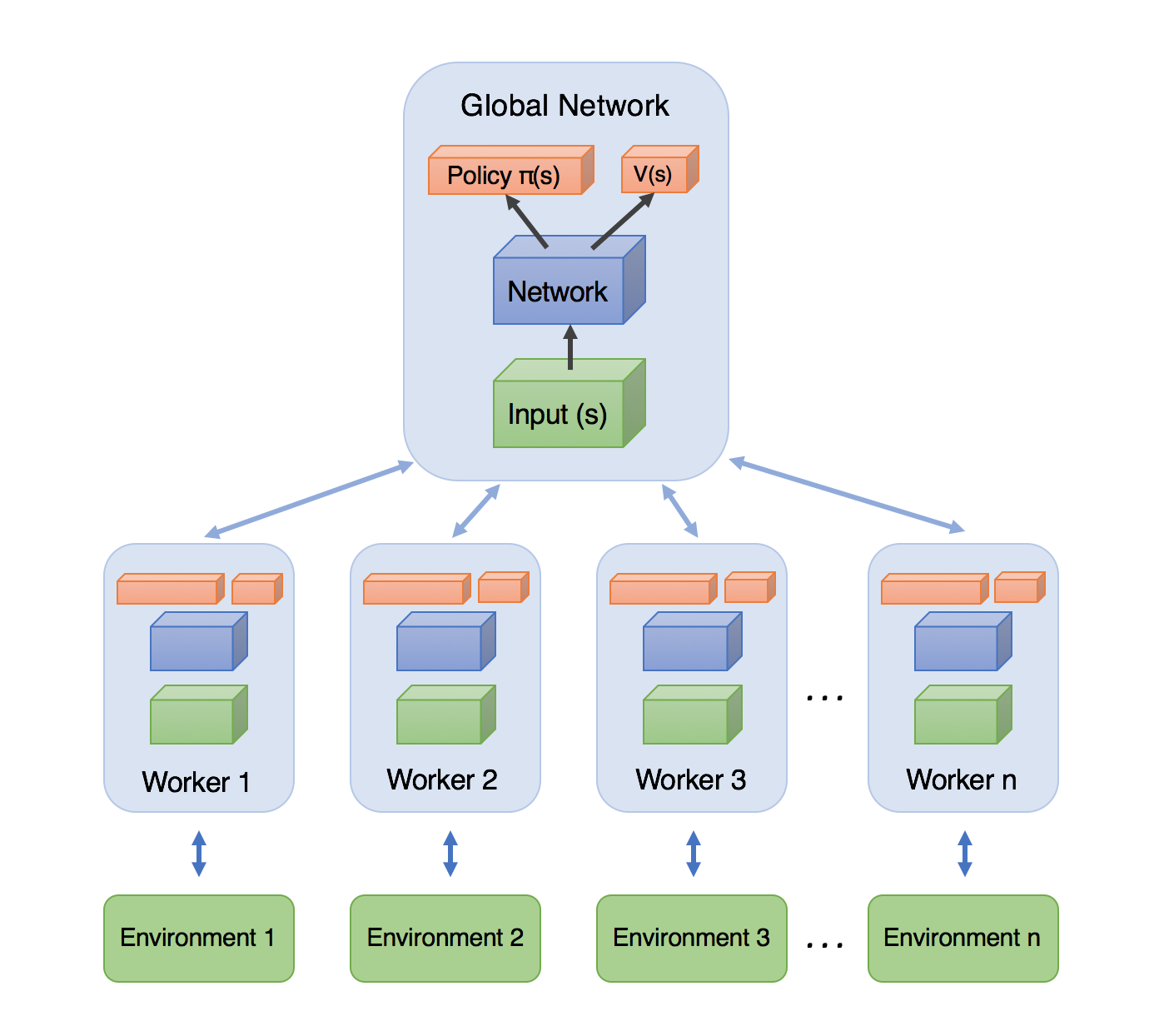
use python’s multiprocessing library to have multiple workers (each one running on a thread) collect episodes, calculate the loss and update the master (global) network, before downloading the new updated parameters
Phil has a good tutorial video here
will probably not implement this one, because A2C with vectorized environments has been empirically shown to be just as good.

Implementation

First, we need to rewrite the updates in terms of losses $\mathcal{L}_{\text{critic/actor}}$ that can be backpropagated in order to use modern Deep Learning libraries.

For the critic, we just want to approximate the true state-values. To do that, we move them closer to the observed return $G_t$, using either a squared error or the Huber-loss, that doesn’t put as much weight on outliers. We can also use some $L_2$ regularization on the Delta of parameters $\Delta \textbf{w} = \textbf{w}_{\text{new}} - \textbf{w}$ to ensure that we don’t update our parameters too much (this is always a good idea in Reinforcement Leraning, because bad policy leads to bad data in the future):

\[\begin{align*} \mathcal{L}_{\text{critic}} &= \| \hat{Q}(s_t,a_t) - \hat{V}(S_t,\textbf{w}) \|_2^2 + \kappa \| \textbf{w}_{\text{new}} - \textbf{w} \|_2^2 \\ &= ( \hat{A}(s_t,a_t) )^2 + \kappa \| \textbf{w}_{\text{new}} - \textbf{w} \|_2^2 \end{align*}\]

I didn’t add the regularization to the implementation yet, because i couldn’t figure out how to implement it in PyTorch so far (you would have to backpropagate the loss first and then calculate the squared $L_2$ norm of the new and old parameters), so treat it as if we set $\kappa=0$ :-( .

Note: Every time this happens and you can’t add the regularization term, just add clip (4Head)

For the actor, we are using the advantage $A(s, a)$ instead of $\delta$ now, which is one of the shown variations. To get our loss, we can just pull in the factor $A(S,A,\textbf{w})$ like this: $a \nabla_x f(x) = \nabla_x a f(x)$ (the factor $A(S,A,\textbf{w})$ doesn’t depend on $\theta$, otherwise this wouldn’t be valid).

Also note that $\gamma^t$ is already baked into the discounted return $G_t$. Discounting makes a lot of sense for many environments, because the action probably has a higher effect short-term and doesn’t matter that much long-term. You should consider your environment carefully here though, because in some cases, for example the game Go, action might have a long-term influence/effect. [6]

For readability, i’ll leave out the $t$ in the subscript in the following formulas, but all $S$, $A$ and $Q$ are in timestep $t$. Lastly notice that we’ll have to negate the entire term to get a loss function, because now instead of maximizing the term, we minimize the negative term (which is the same).

\[\begin{align*} \theta &= \theta + \alpha_\theta A(S,A,\textbf{w}) \nabla_\theta \log \pi(A|S,\theta) \\ &= \theta + \alpha_\theta \nabla_\theta A(S,A,\textbf{w}) \log \pi(A|S,\theta) \\ \\ \Rightarrow \mathcal{L}_{\text{actor}} &= - A(S,A,\textbf{w}) \log \pi(A|S,\theta) \\ &= - [\hat{Q}(s,a) - V(S,\textbf{w})] \log \pi(A|S,\theta) \end{align*}\]

Note that $\hat{Q}(s,a)$ is estimated with a k-step rollout (see section: “Variance vs. Bias tradeoff”). Another choice that we’ll have to make after letting the episode play out is whether we want to update the networks for each timestep or only once. If you chose the latter, you can just sum over all the individual losses to get one loss for the episode:

\[\begin{align*} \mathcal{L}_{\text{actor}} &= - \sum_{t=1}^{T} A(S_t,A_t,\textbf{w}) \log \pi(A_t|S_t,\theta) \\ &= - \textbf{advantages}^\top \textbf{logprobs} \end{align*}\]

Vectorized Environments

In practice, we want to use vectorized environments to get less variance for the loss and thus speed up training (See: Gymnasium docs for vectorized envs). With vectorized environments, we can play k steps with n environments in parallel and just use the mean loss of each sample phase (update every k steps).

If you want to be fancy or use your agent that was trained in simulation in the real world (Sim2Real paradigm), you can also randomize the parameters of your environments to make your agent a little bit more generally capable (domain randomization - see other ressources [11]). This is not difficult to code up (also see gymnasium docs). Be careful though to have enough environments so that your agent doesn’t overfit to certain parameter settings (or create new environments with new parameters every couple of sampling phases).

Example code for domain randomization in the LunarLander-v2 environment:

n_envs = 5
randomize_domain = True

if randomize_domain:
    envs = gym.vector.AsyncVectorEnv([
        lambda: gym.make(
            'LunarLander-v2',
            gravity=np.clip(np.random.normal(loc=-10.0, scale=2.0), a_min=-11.99, a_max=-0.01),
            enable_wind=np.random.choice([True,False]),
            wind_power=np.clip(np.random.normal(loc=15.0, scale=2.0), a_min=0.01, a_max=1.99),
            turbulence_power=np.clip(np.random.normal(loc=1.5, scale=1.0), a_min=0.01, a_max=1.99),
            max_episode_steps=600
        ) for i in range(n_envs)
    ])
    
else:
    envs = gym.vector.make('LunarLander-v2', num_envs=n_envs, max_episode_steps=600)

Note: We have to clip the randomly generated parameters at a min and max point to match the recommended bounds (environment specific). The mean of the gaussians used for generation of the parameters matches the predefined values of the normal gymnasium environment. You can change the scale (variance) to vary the degree of randomization.

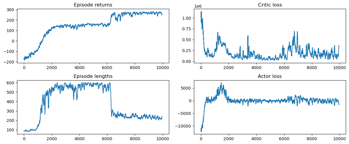
Results

Learning plots

Learned policy showcase (in the LunarLander-v2 environment)

Watch the learned policy (using the A2C implementation) land the spacecraft (you can imagine that it fires real boosters; it’s just easier to show a couple of particles firing, but the physics is the same as if it were real, of course simplified here):

You can actually try to play it yourself, just copy and paste these three lines. I tried and it is actually way harder than it looks. One reason is that you can only fire one booster per timestep – the agent flickers the boosters to gain more balance, but for me that seems pretty hard to do. This is me trying to land it:

(Don’t trust me with landing your rockets…)

…But maybe trust the RL agents that i build :)

Implementation details that i’ve learned from this

retain_graph=True if you want to backward multiple losses though a shared network
loss = a * loss1 + b * loss2 and then just loss.backward() works to update both networks and the shared body at the same time
having a shared network is (at least in my implementation) pretty unstable
Hubert loss (less weight on outliers) is a nice idea in theory, but didn’t really make it better in practice (at least for the environments i tried, here MSE was better)
it works faster on CPU - at least for the small Neural Nets that i tested (probably because data structures are constantly moving between CPU-GPU if you use a GPU.)

Corresponding neuroanatomic structures to Actor and Critic

The functions of the two parts of the stratum (dorsal stratum -> action selection, ventral stratum -> reward processing) suggest that an Actor Critic mechanism is used for learning in our brains, where both the actor and the critic learn from the TD-Error $\delta$, which is produced by the critic. A TD-Error $\delta > 0$ would mean that the selected action led to a state with a better than expected value and if $\delta < 0$, it led to a state with a worse than average value. An important insight from Neuroscience is that the TD-Error corresponds to a pattern of dopamine neuron activations in the brain, rather than being just a scalar signal (in our brain, you could look at it as a vector of dopamine-neuron activity). These dopamine neurons modulate the updates of synapses in the actor and critic structures.

\[\begin{align*} \text{TD-Error} \; \delta \; &\hat{=} \; \text{Activation pattern of dopamine neurons} \\ &\hat{=} \; \text{experience - expected experience} \end{align*}\]

The following image shows the corresponding structures in mammalian brains and how they interact.

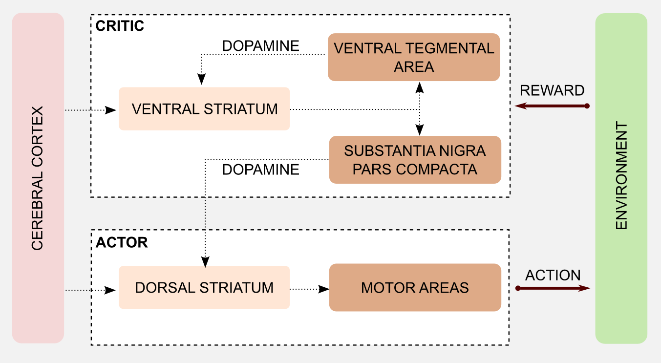
Illustration from Massimiliano Patacchiola's blog [9]

Dopaminergic circuit with labels for the corresponding Actor-Critic components

Experiments show that when the dopamine signal from the critic is distorted, e.g. by the use of cocaine, the subject was not able to learn the task (because the dopamine/error signal for the actor is too noisy).

Final remark: Clean formalism

Reinforcement learning notation sometimes gets really messy and unpleasent to look at, to the point where it can be hard to absorb the important pieces of information. For this reason i think it is usually better to omit some formalism and instead write clean looking formulas for the sake of readability, if the context of writing allows it (i.e. you are not writing a scientific paper). A piece that you can usually leave out if it is clear what we are referring to is $\theta$ in the subscript.

References

Illustration of the Neural Net architecture with a shared body taken from here.
Stackexchange post: Why we are using $\gamma$ as discounting to update the actors parameters $\theta$
Sutton & Barto: Reinforcement Learning, An introduction (second edition)
Hado van Hasselt: Lecture 8 - Policy Gradient
HHU-Lecture slides: Approximate solution methods (for the semi-gradient definition)
Pieter Abbeel: L3 Policy Gradients and Advantage Estimation (Foundations of Deep RL Series)
Daniel Takeshi’s blog: Notes on the Generalized Advantage Estimation Paper
PyTorch docs: HuberLoss
Mnih et. al. : Asynchronous Methods for Deep Reinforcement Learning
Jonathan Hui: GAE
higgsfield’s “RL-Adventure-2: Policy Gradients” GitHub repository (Actor-Critic, GAE, PPO, ACER, DDPG, TD3, SAC, GAIL, HER) – took this as reference for writing the GAE calculation
John Schulman, Philipp Moritz, Sergey Levine, Michael Jordan, Pieter Abbeel: High-Dimensional Continuous Control Using Generalized Advantage Estimation (GAE paper)
David Silver, Lecture 7: Policy Gradient (lecture slides)
Stable Baselines3: A2C (implementation used for reference for the entropy bonus and to check if my GAE implementation is correct)

Pointers to other ressources

Chris Yoon: Understanding Actor Critic Methods and A2C
Richard Sutton: Actor-Critic Methods
Berkeley lecture slides
CS885 Lecture 7b: Actor Critic
Actor Critic blogpost with illustrations and eligibility traces
TD(0) Actor Critic code
PyTorch Actor Critic implementation.
Nice ressource on A2C (1-step and n-step) with code here.
Massimiliano Patacchiola: Dissecting Reinforcement Learning-Part.4: Actor-Critic (AC) methods (+ Correlations to Neuroanatomy)
Machine Learning with Phil: Multicore Deep Reinforcement Learning - Asynchronous Advantage Actor Critic (A3C) Tutorial (PYTORCH)
Josh Tobin, Rachel Fong, Alex Ray, Jonas Schneider, Wojciech Zaremba, Pieter Abbeel: Domain Randomization for Transferring Deep Neural Networks from Simulation to the Real World